
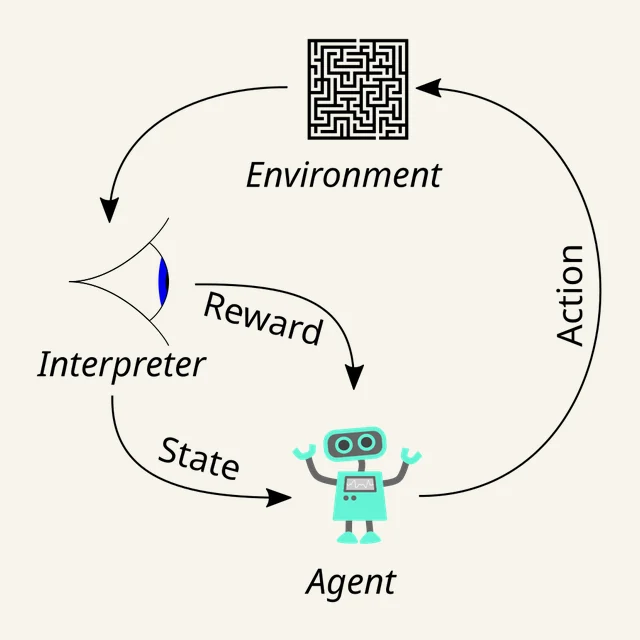
When a reinforcement learning (RL) experiment fails, inspect the task, hidden context, training distribution, episode boundary, data pipeline, and evaluation protocol before tuning the optimizer. This article merges the existing evergreen tutorial with two historical Obsidian notes on open-world RL, meta-RL, and pre-trained perception, then rechecks the combined claims against primary sources. It focuses on reasoning and tests that remain useful across libraries; tool links were last verified on 2026-08-08.
Define the experimental contract before the algorithm
Deep Q-Network (DQN), Soft Actor-Critic (SAC), Proximal Policy Optimization (PPO), model-based RL, offline RL, and meta-RL are families of methods. An algorithm optimizes the specified return. The research objective may concern safety, completion time, generalization, interaction cost, or several competing criteria. Rewards, evaluation metrics, and resource budgets must connect that objective to the experiment; otherwise training can optimize the wrong proxy.
I freeze a one-page experimental contract before implementing an algorithm:
| Part | Question that must be answered |
|---|---|
| Decision process | What are the observation, action, reward, termination, time scale, and sources of randomness? |
| Task distribution | How are training, validation, and test tasks generated, and which factors are deliberately held out? |
| Resource budget | How do environment steps, real interactions, wall-clock time, compute, and tuning trials count? |
| Evaluation unit | Is an episode, task, seed, or complete training run the independent unit? |
| Baselines | Which methods represent random behavior, a strong task-specific solution, adjacent work, and an idealized upper bound? |
| Failure policy | How are crashes, timeouts, invalid actions, numerical errors, and missing results handled? |
This contract states the evidence required to support a conclusion. Its constraints also guide every later method choice.
Specify the decision problem first
MDP, POMDP, and what the agent can observe
A Markov decision process (MDP) is commonly written as $(\mathcal{S}, \mathcal{A}, P, R, \gamma)$. At time $t$, the environment is in state $S_t$, the agent chooses $A_t$, and the environment draws the next state and reward from its transition process. The discounted return is
\[G_t = \sum_{k=0}^{\infty} \gamma^k R_{t+k+1}.\]The Markov property is a claim about a chosen state representation: conditional on that representation and the action, the distribution of the next state and reward no longer depends on earlier history. The latest sensor reading may fail this condition. If a camera frame hides velocity, a delayed actuator depends on earlier commands, or an opponent has private information, the observation is generally only a partial view of the state. The problem is then better described as a partially observable MDP (POMDP).
Before selecting an algorithm, write down:
- the observation available at decision time, including units and bounds;
- the action space and any feasibility constraints;
- the transition timing—when an action takes effect and when its consequence is observed;
- the reward and the real-world objective it is intended to represent;
- terminal states, external cutoffs, and the discount or finite horizon.
If the latest observation is insufficient, add a justified history window, recurrent state, state estimator, or belief representation. Do not expect a larger feed-forward network to reconstruct information that was never observed.
The standard foundation remains Sutton and Barto’s Reinforcement Learning: An Introduction. Its definitions are more durable than framework-specific tutorials.
State may hide the task
The vector emitted by an environment is not automatically a sufficient state. If the same observation requires different actions under hidden rules, goals, or dynamics, the agent faces partial observability. Meta-RL makes this problem explicit: an agent must infer the current task from limited interaction and then control accordingly. PEARL separates task inference from control and represents uncertainty with a probabilistic context variable. A task representation should explain why the same observation calls for another behavior in this task and preserve the task differences relevant to action selection.
Offline data can also entangle task identity with the collection policy. If one task happens to be collected by a stronger behavior policy, an encoder may mistake “these trajectories look better” for task identity. Robust Task Representations directly studies this task–behavior-policy confounding and representation robustness when behavior-policy distributions change at test time.
State and task representations need at least three counterfactual checks:
- Same task, different behavior policies: does the representation remain close, and can the policy still adapt?
- Different tasks, similar trajectory quality: can it separate factors that change optimal behavior?
- Shuffled history or context: is the performance change caused by task information, temporal information, or merely data volume?
Clusters in a two-dimensional projection show that an encoder formed groups; the counterfactual checks above are still needed to establish that it “learned the task.”
Episode boundaries are part of the model
There are two different reasons a rollout can stop:
- Termination: the MDP reaches a terminal condition, such as success, failure, or a finite-horizon endpoint included in the task definition.
- Truncation: data collection stops for a reason outside the MDP, such as a wrapper’s time limit, a simulator interruption, or an external safety monitor that deliberately ends collection outside the task definition. If crossing a safety bound is itself a task-defined failure, that event is a termination instead.
This distinction changes a bootstrapped target. For a one-step value target,
\[y_t = R_{t+1} + \gamma \left(1-\mathbb{1}[\text{terminated}_t]\right)V(S_{t+1}).\]An external truncation normally resets the environment but does not by itself erase the continuation value. Conversely, a time limit that is genuinely part of a finite-horizon MDP is a termination; the remaining time must be represented in the observation if it affects the transition dynamics. The Gymnasium time-limit tutorial gives the current operational distinction.
Implement the environment contract
Use the current Gymnasium API deliberately
The current Gymnasium Env interface separates reset information, termination, and truncation:
observation, info = env.reset(seed=seed)

while True:
    action = policy(observation)
    next_observation, reward, terminated, truncated, info = env.step(action)

    replay.add(
        observation,
        action,
        reward,
        next_observation,
        terminated,
        truncated,
    )

    if terminated or truncated:
        observation, info = env.reset()
    else:
        observation = next_observation
Store terminated and truncated separately unless the learning code has already converted them into an explicit bootstrap mask. Collapsing both into an old done flag is a common way to bias value targets.
Test semantics before learning
A random policy should be able to run thousands of steps without invalid observations, illegal rewards, or inconsistent episode statistics. Add tests for:
- observation shape, dtype, finiteness, units, and declared bounds;
- action clipping or rejection and every boundary action;
- deterministic transitions under a fixed simulator state when determinism is expected;
- reward decomposition and cumulative return on a hand-computed trajectory;
- every termination and truncation path;
- wrapper order, because wrappers may alter observations, rewards, and episode length;
- vectorized environments, especially per-worker reset and final-observation handling.
An environment checker can catch interface errors. Verifying that the reward describes the intended task requires a separate test. Keep a tiny deterministic environment with a known solution as a regression test for the learning code.
Define the distribution beyond a fixed task
A single fixed level can show whether an agent memorizes one solution but says little about transferable capability. Open-world and procedurally generated environments shift the object of study to a task distribution: goals, maps, opponents, resources, rule combinations, and horizons vary, and training cannot enumerate every future case.
The XLand open-ended learning work treats the universe of tasks as part of the research object and notes that progress itself becomes difficult to measure across many incomparable tasks. Procgen uses procedurally generated levels to separate training efficiency from generalization to unseen levels. Together they show why an open task setting cannot be summarized by average return on the training distribution.
An interpretable protocol first decomposes the task space into axes, then defines hold-outs:
- compositional hold-out: skills A and B appear in training but never in their test combination;
- parameter extrapolation: speed, scale, noise, or terrain lies outside the training range;
- rule shift: observations look familiar while the objective or dynamics change;
- horizon shift: local skills stay fixed but the dependency chain becomes longer;
- behavior-policy shift: the collection distribution changes for offline or meta-learning data.
Evaluation should report training-distribution, interpolation, genuinely held-out composition, and diagnostic-probe results separately. If the task generator evolves during training, preserve its version and sampling weights; otherwise “more open” is an adjective that cannot be reproduced.
A long horizon is more than a larger discount factor
Long-range planning combines delayed reward, sparse successful behavior chains, effects of early actions that surface much later, and high-level goals that invoke several low-level skills. Increasing the discount factor changes return weighting but does not create discoverable subgoals or reliable memory.
I divide long-horizon capability into three tests:
- Skill layer: can navigation, interaction, evasion, or resource collection be completed in isolation?
- Composition layer: when two known skills appear in a new order, at which interface does failure occur?
- Planning layer: with sparse intermediate reward, can the agent preserve a goal, recover from failure, and choose an alternative route?
Hierarchical policies, memory models, world models, and sequence modeling may all help, but they address different bottlenecks. Horizon truncation, shuffled history, provided or removed subgoals, and substituted low-level skills are useful ablations; without them, “the model is larger” can be mistaken for “the model plans.”
Choose learning or evaluation methods from constraints
Algorithm names should come after the data-generating process. Action type narrows the options, but interaction cost, parallelism, partial observability, safety constraints, and the availability of logged data often matter more.
| Situation | Reasonable starting method | Main cost or risk |
|---|---|---|
| Small, known finite MDP | Dynamic programming or tabular temporal-difference methods | State-space growth |
| Discrete actions with an online simulator and reusable transitions | Value-based off-policy methods such as the DQN family | Exploration and value overestimation; replay assumptions |
| Continuous actions where environment steps are expensive | Off-policy actor–critic methods such as SAC or Twin Delayed Deep Deterministic Policy Gradient (TD3) | More coupled components and sensitivity to scale |
| Many parallel simulators and a simple, well-tested baseline | On-policy policy-gradient methods such as PPO | Discards old policy data and can require many interactions |
| A fixed log, with the goal of learning a new policy | Offline RL methods matched to the data coverage and deployment constraints | Distribution shift and poor action coverage cannot be repaired by optimization alone |
| A fixed log, with the goal of evaluating an existing policy | Off-policy evaluation matched to assumptions about behavior policies and coverage | Unsupported actions and unknown propensities can make the estimate unidentifiable or high-variance |
| A trustworthy model is available or can be learned and validated | Planning or model-based RL | Model bias compounds along imagined rollouts |
The table provides an engineering starting heuristic. Primary entry points include the original work on DQN, TD3, SAC, and PPO, plus an offline RL tutorial and review and a primary example of doubly robust off-policy evaluation. Read their assumptions and experimental protocols before transferring a method. The Stable-Baselines3 algorithm guide can cross-check current action-space support and implementation details. Start with one mature baseline and a budget small enough to debug. Add recurrence, distributional value estimation, prioritized replay, auxiliary losses, or model learning after the simpler system establishes a trustworthy signal.
On-policy and off-policy describe how updates relate to the policy that generated the data. On-policy methods limit reuse to data close to the current policy. Off-policy methods can reuse older data, usually improving sample efficiency, but must manage mismatch between the behavior distribution and the current target. Neither label implies that one family is always more stable or more accurate.
Design rewards and scales as part of the experiment
Optimize the intended outcome
A dense reward can make credit assignment easier. Every shaping term changes what is easy to optimize and may open a shortcut. Reward hacking is the general failure mode in which the agent scores well under the written objective without accomplishing the designer’s intent.
Use this process:
- define success metrics and retain independent metrics that are not training rewards;
- test the reward on hand-designed good, bad, stalled, and adversarial trajectories;
- log every reward component separately;
- inspect high-return trajectories alongside scalar curves;
- evaluate under environment variations that make known shortcuts fail;
- when violations are unacceptable, use explicit constraints or runtime protections—such as action masks, safety shields, constrained optimization, or independent monitors—and treat a soft reward penalty as auxiliary.
Potential-based shaping has a specific policy-invariance result under its assumptions. A shaping term of the form
\[F(s,a,s') = \gamma\Phi(s') - \Phi(s)\]can preserve optimal policies while altering learning signals; arbitrary progress bonuses do not inherit that guarantee. The guarantee also requires consistent treatment of episode boundaries: finite episodic implementations commonly set the terminal-state potential to zero, while an external truncation must not be silently treated as a terminal state. See Ng, Harada, and Russell’s reward-transformation paper.
Make observation, action, and reward scales explicit
Many common function approximators and optimization configurations are harder to train when feature scales differ by many orders of magnitude. Record preprocessing as part of the environment contract:
- standardize unbounded continuous observations using statistics collected only from training data;
- represent categorical variables with an encoding that introduces no arbitrary distances;
- expose continuous policy actions on a simple symmetric range when possible, then transform them to actuator units;
- keep clipping visible and count how often it occurs;
- log raw task return even when the learner uses normalized or scaled rewards.
Changing reward scale, discount, or action transformation can change optimization and sometimes the effective objective, so record them explicitly as experiment parameters.
Architecture rules are conditional
The suitability of convolution, pooling, and batch normalization depends on the observation and training distribution. Choose inductive biases from those conditions:
- convolution is useful when local spatial structure is meaningful;
- pooling helps when the discarded location detail is genuinely irrelevant, but hurts tasks requiring precise coordinates;
- batch normalization can be awkward when samples are correlated, replay data mix policies, batches are small, or acting and learning statistics differ; it can still work when statistics and train/evaluation modes are controlled;
- recurrent or attention-based models help only when the supplied history contains information needed to resolve partial observability.
The precise term is “orthogonal initialization.” It is one possible parameter-initialization choice and carries no convergence guarantee. Whenever the architecture changes, compare it under the same environment steps, preprocessing, optimizer budget, and seed protocol.
Visual pre-training is a transfer hypothesis to measure
Learning control from pixels can spend much of the interaction budget on perception. A pre-trained encoder may reduce that cost; each combination of pre-training method, data, and update policy requires its own cross-domain validation. Pre-trained Vision Models for Control compares pre-training methods, augmentation, and feature levels across several control domains; ATC decouples representation learning from policy learning and examines frozen encoders, multi-task data, and temporal contrastive objectives; the broader VC-1 embodied-task evaluation further shows that strong average performance still requires validation on each downstream task.
A minimum pre-training experiment compares the following under the same budget:
| Condition | How the encoder is obtained | How it changes during RL | Main identification target |
|---|---|---|---|
| From scratch | Random initialization | End-to-end with the policy | What current-task data alone can learn |
| Frozen pre-training | External or multi-task data | Fully frozen | Whether a ready-made representation is directly usable |
| Fine-tuned pre-training | The same pre-trained checkpoint | All or selected layers update | Whether adaptation repairs domain mismatch |
| Frozen and online feature fusion | A pre-trained branch plus a task branch | Independent or partially updated branches | Whether general perception and task information complement one another |
All four should share the policy algorithm, environment-step budget, action inputs, seeds, and evaluation tasks. Beyond final return, report early sample efficiency, wall-clock and memory cost, out-of-domain tasks, task-inference stability, and sensitivity to feature level. Freezing, augmentation, batch composition, and non-stationary data interact, so transfer claims require the complete controlled comparison.
Treat replay as a changing dataset
Replay requires an update rule that supports off-policy data, and buffer capacity trades off:
- coverage: retaining rare outcomes and different parts of the state space;
- freshness: avoiding domination by behavior from policies that are no longer relevant;
- memory and throughput: storing images or long sequences may become the bottleneck;
- sequence integrity: recurrent methods may need contiguous segments and burn-in.
Measure the age distribution, reward or terminal-event frequencies, and sampling ratio. If the environment or task changes, version the data or clear the buffer; otherwise the learner may silently mix incompatible transition processes.
Prioritized experience replay (PER) samples transitions using a priority such as temporal-difference error and applies importance weights to reduce sampling bias. The original PER paper presents a replay scheme used throughout training. PER may improve learning efficiency, but noisy rewards, outliers, stale priorities, and reduced diversity can make a high error a poor proxy for usefulness. Use uniform replay as a control, log effective sample weights, and tune priority strength.
Separate training, selection, and evaluation
A training curve provides diagnostic evidence. A final estimate also requires three distinct environment roles:
- training environments collect updates and fit normalization statistics;
- validation environments choose checkpoints and hyperparameters;
- test environments are used only for the final reported comparison.
Keep wrappers and task definitions equivalent where intended. Evaluation uses a frozen copy of the training normalization statistics and never updates them; its data stream remains isolated from replay. Before running, use the deployed policy to decide whether evaluation uses deterministic actions, samples from a stochastic policy, or reports both.
An evaluation report should include:
- environment and wrapper versions, code revision, hardware, and numerical settings;
- the number of environment interactions and other material compute budgets;
- multiple independent training seeds and evaluation episodes for each;
- per-seed returns and episode lengths, failures, constraint violations, and task-specific metrics;
- a predefined checkpoint-selection rule and baseline implementations under the same budget;
- interval estimates or bootstrap uncertainty plus a predefined aggregate.
Deep Reinforcement Learning that Matters documents how implementation and reporting choices change conclusions. Deep RL at the Edge of the Statistical Precipice shows why point estimates from a few runs are fragile and motivates interval estimates, performance profiles, and robust aggregate metrics. PyTorch also warns that exact reproducibility is not guaranteed across releases, platforms, or CPU and GPU execution; its reproducibility notes explain how to control random sources and request deterministic algorithms when the debugging benefit justifies the performance cost.
Debug in layers
When learning fails, change one layer at a time:
- Environment: replay a hand-authored trajectory and verify every observation, reward component, boundary, and metric.
- Data: inspect sampled batches, bootstrap masks, action ranges, sequence boundaries, and replay age.
- Loss: test targets on small tensors; check broadcasting, detached target networks, signs, reductions, and importance weights.
- Optimization: log gradient and parameter norms, NaNs, clipping frequency, entropy or exploration noise, and update-to-data ratio.
- Learning signal: solve a bandit or tiny deterministic MDP, then a standard small environment, before the full task.
- Evaluation: run random, constant-action, scripted, and previous-policy baselines through exactly the same evaluator.
PyTorch provides gradcheck, autograd anomaly detection, and torch.profiler. Use assertions and structured logs for durable diagnostics; reserve Python’s print() for a narrow local probe.
Evaluate self-play as a population
Self-play makes the data distribution move because every policy update changes part of the environment. Evaluating only against the latest opponent can hide forgetting and cycles. A simple “higher policy beats lower policy” ladder assumes transitivity, but many games admit rock–paper–scissors-style relations: $A$ beats $B$, $B$ beats $C$, and $C$ beats $A$.
Use a payoff matrix across current and historical checkpoints, fixed scripted opponents, and independently trained populations. Report role or side asymmetry, exploitability when it can be computed, and performance against withheld opponents. Sample opponents from a population or mixture so that training does not overfit one moving target. Alpha-Rank is one research example of population-level evaluation for multi-agent interactions. AlphaZero demonstrates successful self-play in perfect-information zero-sum games. Applying that conclusion to other environments requires separate evaluation of naive latest-policy self-play; see the AlphaZero paper.
Use libraries as replaceable instruments
As of 2026-08-08, useful entry points include:
- Gymnasium for environment interfaces and wrappers;
- PyTorch for differentiable models, optimization, and diagnostics;
- Stable-Baselines3 for compact reference implementations and experiment utilities;
- RLlib for distributed sampling and multi-agent workloads;
- ElegantRL as another implementation source to inspect.
Record the exact package versions and verify behavior against their tests and documentation. A library can provide a correct interface and still leave task semantics, reward validity, hyperparameter budgets, and statistical claims to the experimenter. The lasting workflow is: specify the decision process, test the environment, establish a simple baseline, inspect the data, separate evaluation, quantify uncertainty, and then add algorithmic complexity.
A research checklist
Before believing an RL curve, confirm that:
- task, state, hidden context, and evaluation metrics are defined separately;
- generation and hold-out rules for training, validation, and test tasks are reproducible;
- termination, truncation, and bootstrap-mask semantics have been tested on a hand-built trajectory;
- long-horizon difficulty is decomposed into skill, composition, and planning;
- a pre-trained encoder has budget-matched from-scratch, frozen, fine-tuned, or fusion controls;
- reward shaping has not changed the real objective without a check;
- replay capacity, sampling, age, and behavior distribution are all recorded;
- baselines include random behavior, a strong task-specific method, and adjacent research routes;
- curves, failures, and uncertainty are retained for every task and seed;
- each central claim has an ablation or distribution shift capable of falsifying it.
This checklist clarifies the problem before algorithm selection and keeps conclusions open to interrogation after a curve appears.
Comments
Comments are public and stored in GitHub Discussions. This page connects to giscus.app and GitHub and sends the current page path only after you show comments manually or enable automatic loading. The first load is about 0.13 MB; actual usage varies with comment content. Do not include private information.